Step-by-step application setup

Setting up a data-assimilation framework for a model is a difficult task. Several things contribute to the complexity. The dynamical models are often complex software packages with many options. In addition, we add (real) observed data and blow up the number of computations and data by an order of 100. Another problem is related to our way of using the models in a data-assimilation framework. For sequential data-assimilation algorithms, such as the Ensemble Kalman Filter (EnKF) or 3D-VAR, we often perform (short) model runs and update the parameters or state of the model between these short runs. However, the used simulation models are often not developed to be applied in this way.

Many users are struggling to get things to work because they want to do too much too soon. A recipe for failure is to attempt to set up your data-assimilation system for a real (big/huge) model with real data in one go. On this page, we describe some intermediate steps that can be taken to set up and test your application. There is no one-size-fits-all approach, but we try to present a recipe that you can use or adapt to your own needs. In between, there are useful tips and ideas.

For simplicity, we assume that the user uses a black-box coupling and wants to set up a data-assimilation system using a sequential data-assimilation algorithm e.g. a flavor of the Ensemble Kalman filter.

Preparation

Start small

Setting up a data-assimilation system involves many steps and challenges. We advise not to focus on your final setup directly, which will involve real observations and probably a large simulation model. The last thing you will introduce is your real observations. You need their specifications e.g. location, quantity, quality, and sampling rate in an early stage since it is an important aspect of your system, but the measured values will not be used the first 80% of the time. To set up and test your framework it is best to use generated/synthetic data that you understand. We will explain this in more detail in the paragraph about setting up twin experiments below.

If possible, make various variations of your model. Start with a very, very simplified model that runs blisteringly fast and only incorporates the most basic features. When you have everything working for this small model, you move toward a more complex model. The number of steps you need to take to implement your full model depends on many aspects. Making these “extra” small steps is time well spent, and in our experience, you will save a lot of time in the end.

Create experiments with one group of observations at a time when you want to assimilate observations of various quantities and/or sources. You will learn a lot about the behavior of your model when assimilating these different types of observations, and it is much easier to identify which kind of observations might cause problems, like model instabilities.

Check the restart of a model

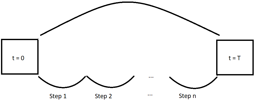
To use a programmed model as part of a sequential data-assimilation algorithm, it should have a proper restart functionality. This makes it possible to split up a long simulation run into several shorter ones. The model will write the internal state to one or more restart files at the end of each run. This will contain the model state \(x\), but often some other information as well, e.g. the information on the integration step size, computed forcing, etc. The restart information will be read from disk at the start of the next run. There should be no differences in the result between the restarted simulations and the original simulation when the restart is implemented correctly.

To check whether the restart functionality of your model is working properly, run a simulation in one go (using the algorithm Simulation) and perform the same simulation with several restarts (using the algorithm Sequential simulation). It is always best to choose the same interval between the restarts as the assimilation interval you plan to use in your data-assimilation framework.

Note: In case your model software is already coupled to OpenDA it is still very important to check whether for your particular model setup the restart functionality works. Your model may be using features that impact the restart and have not been catered to in the original coupling to OpenDA.

Example of a proper restart functionality

Unfortunately, the restart functionality of models is often not perfect. When that is the case you have to look at how bad it is. Here is a list of issues we have seen in the past that might cause differences:

Loss of precision: some precision can be lost in reading and writing values from the restart files (e.g. computations are in double precision but restart is in single precision). When we expect that the model updates of the data-assimilation algorithm are much larger than this loss of precision, it is only annoying (it makes testing/comparing/debugging more difficult) but no showstopper.
Incomplete restart information: at some point in the model history some functionality has been added but the developers forgot to incorporate the relevant new (state) information in the restart file.
Imperfect by design: sometimes, the developers never intended to have a perfect restart functionality, which means the results are not exactly the same as without the restart. Writing a correct restart functionality is often far from easy.

Some tips when you notice the restart is imperfect:

Experiment with a simplified model. Switch features on and off to figure out where the differences are originating from.
Does your model have automatic integration steps? Check the initial integration time steps for your restarted model. Can you run your model with constant integration time steps?
How is the model forcing defined? Does the model interpolate your forcing input data? Changing the model time steps might fix your problems.
Contact the developers of the code. With some luck, they are willing to help you.

In the end, you have to figure out whether the errors in the restart are acceptably small. When the deviation between the original run and a run with restarts is much smaller than the expected impact of your data assimilation you might be OK.

Uncertainty of your model

For the ensemble-based algorithms, you need to have an ensemble that statistically represents the uncertainty in your model prediction. There are various ways to set up your ensemble.

When your model is dominated by chaotic behavior, e.g. for most ocean and atmospheric models, you can generate an initial ensemble by running the model for some time and taking various snapshots of the state. Another approach is to set up an ensemble of model states with some initial perturbation. Then run the ensemble long enough for the chaotic behavior to do its work and use that as the initial ensemble of your experiment.
When the uncertainty is dominated by the forcing, e.g. coastal-sea, river, air-pollution, run-off and sewage models, you have to work on describing the uncertainty, including time and spatial correlations of these forcings.
When the uncertainty is in the parameters of the model, e.g. groundwater and run-off models (and we are not planning to estimate them), you can carefully generate an ensemble of these parameters that represents their uncertainty. Then you set up your ensemble in such a way that each member has a different set of parameters. Be aware that this setup is not suited for all flavors of EnKF, since the model state after the update must in some sense correspond to the perturbed set of model parameters!

Combinations of the above are possible as well. It is a good investment of time to generate and explore your (initial) ensemble. Note that the filter can only improve your model based on the uncertainty (subspace) of your ensemble. When important sources are not captured by your ensemble, the filter will not be able to perform well.

Finally, your model may have time-dependent systematic errors. We often found it useful to add an artificial forcing to the model to describe these model errors.

We will explain here how these experiments can be carried out using OpenDA.

Twin experiments

In real-life applications, we use data assimilation to estimate the true state of the system. Unfortunately, we do not know the true state and that makes it difficult to test your data-assimilation system. You can set up a so-called twin experiment to overcome this problem and test your system in a controlled way. The observations in a twin experiment are generated by a model run with a known internal perturbed state or added noise. The perturbation should correspond to the specified uncertainty of your ensemble.

Note: Do not use the mean (or deterministic run), because that realization is special. The true state is known in the twin experiment and has the dynamics of your model. This makes it easy to investigate the performance of your data-assimilation framework. The Sequential simulation algorithm in OpenDA is a useful tool for creating your twin experiment.

Simulation algorithms

OpenDA implements several algorithms that can be used to gradually grow from a simulation model to a data-assimilation system.

Simulation algorithm

Running the algorithm org.openda.algorithms.Simulation is equivalent to running the model stand-alone. The only difference is that it runs from within OpenDA. It allows you to test whether the configuration is handled correctly and whether the output of the model can be processed by OpenDA.

Sequential simulation algorithm

The algorithm org.openda.algorithms.kalmanFilter.SequentialSimulation is again equivalent to running the model by itself. However, this time the model is stopped at each moment at which we have observations (or at predefined intervals). For each observed value, the corresponding value as predicted by the model is written to the output.

The purpose of this algorithm is twofold:

Check whether the restart functionality of the model within the OpenDA framework is working correctly. This is done by comparing the results to a normal simulation.
In addition, it is also used to create synthetic observations for a twin experiment. You set up observations with arbitrary values but with the location and time you are interested in. After you have run this algorithm, you can find the model predictions that you can use for your synthetic observations. Do not forget to add noise to the generated observations. The noise must be of the order of the measurement error when collecting ‘real’ data.

Sequential-ensemble simulation

The sequential-ensemble simulation algorithm (org.openda.algorithms.kalmanFilter.SequentialEnsembleSimulation) will propagate your model ensemble without any data assimilation. This algorithm helps you study the behavior of your ensemble. How is explicit noise propagated into the model? How is the initial ensemble propagated? At the same time, it is interesting to study the difference between the mean ensemble and your model run. Due to nonlinearities, your mean ensemble can behave significantly differently from your deterministic run.

Basic assimilation algorithms

Ensemble Kalman filtering

Next, it is time to start filtering. Therefore, Ensemble Kalman filtering can be used (org.openda.algorithms.kalmanFilter.EnkF), but other algorithms, e.g. DEnKF or EnSR, are also possible. Start with a twin experiment so that you know that there are no artifacts in the observation data. Start small! First, assimilate a small number of observations and take the ones that may have a lot of impacts. Then start adding observations and see what happens. When you want to assimilate observations from various quantities or qualities, first investigate their impact as a group and only mix observations in the final steps.

Next steps

There are various methods and options that can help to improve the performance of your assimilation. To improve the performance you can try to use a pre-computed steady-state Kalman gain (org.openda.algorithms.kalmanFilter.SteadyStateFilter) or use parallel computing to propagate the ensemble in parallel. Spurious correlations can be catered to using localization techniques, which are available on most ensemble-based algorithms.